"""
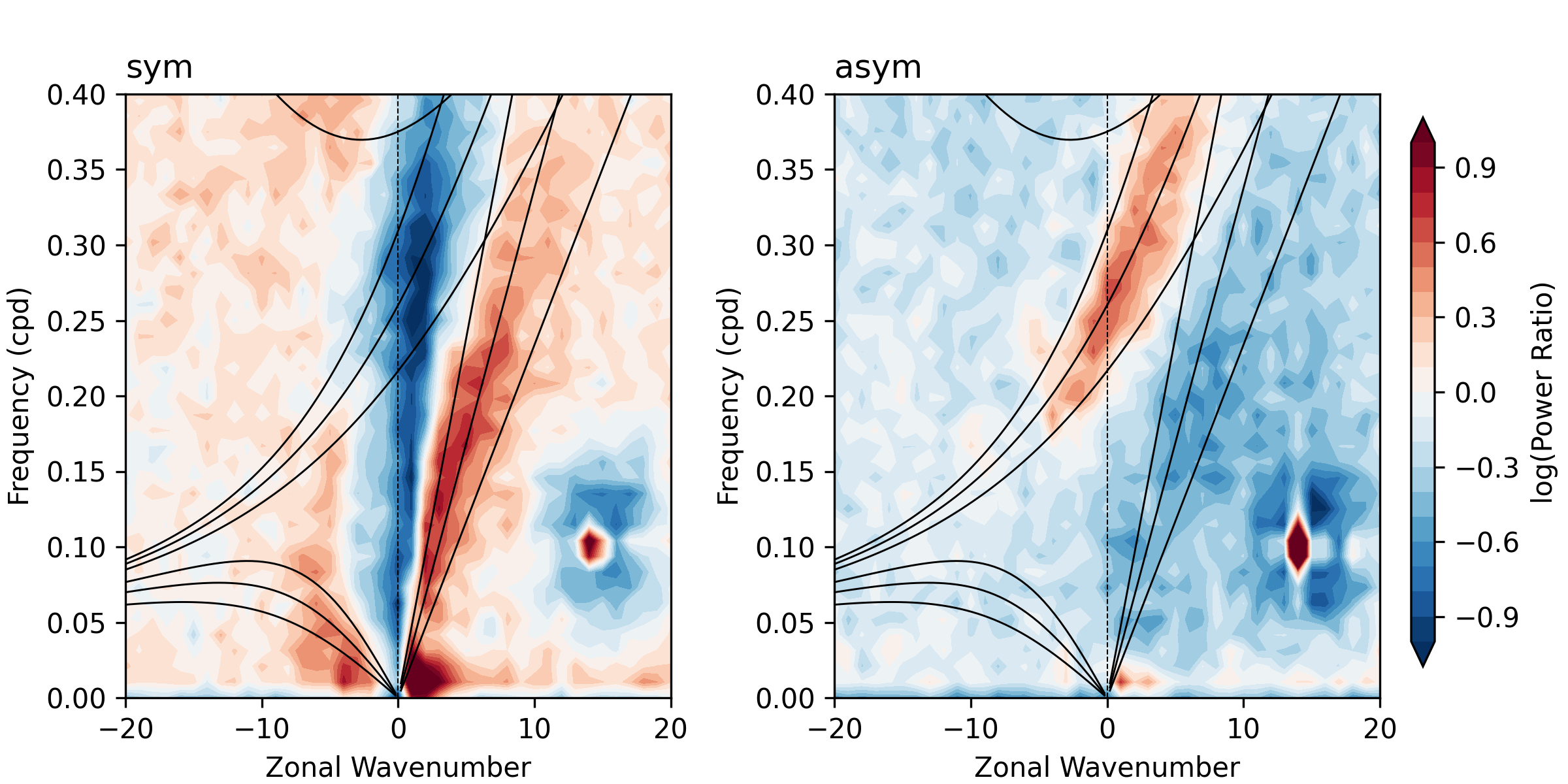
画 OLR 的 WK99 频谱图,并叠加赤道波的频散曲线
"""
import matplotlib.pyplot as plt
import xarray as xr
import numpy as np
import moisten_ew as mew

# 加载数据,并选择南北纬20度以内
data = xr.open_dataset("~/Documents/equator_waves/data/olr.day.mean.nc").olr.sel(
    lat=slice(20, -20),
    time=slice("2000", "2020")
)

# 计算WK99频谱,返回一个 xarray Dataset 对象
res = mew.wk99_spectrum(data, 'lon', 'lat', 'time')

# 选择波数在 -20 到 20 之间,频率在 0 到 1 之间的数据用于画图
res = res.sel(wavenumber=slice(-20, 20), freq=slice(0, 1))


# 画频散曲线
waves = [
    mew.EquatorialWave.IGW,
    mew.EquatorialWave.MRGW,
    mew.EquatorialWave.KELVIN_WAVE,
    mew.EquatorialWave.ERW
]
wavenumber = np.linspace(-20, 20, 100) * mew.unit('zonal_wavenumber')

# 画图
fig = plt.figure(figsize=(8, 4))
gs = fig.add_gridspec(1, 2, wspace=0.3, right=0.88, left=0.08)
for i in range(2):
    ax = fig.add_subplot(gs[0, i])

    # 画与背景的比值
    d = res.spec_ratio.isel(type=i)

    c = ax.contourf(d.wavenumber, d.freq, np.log(d),
                cmap='RdBu_r', levels=np.linspace(-1, 1, 21),
                extend='both')
    # 画频散曲线
    for wave in waves:
        for h in [12, 25, 50]:
            omega = mew.angular_frequency(
                wave, wavenumber, n=1, equivalent_depth=h
            )
            freq = omega/(2*np.pi)  # from rad/day to 1/day

            ax.plot(
                wavenumber, freq, color='k', lw=0.7
            )

    ax.set_ylim(0, 0.4)
    ax.axvline(0, color='k', lw=0.5, ls='--')
    ax.set_xlabel('Zonal Wavenumber')
    ax.set_ylabel('Frequency (cpd)')
    ax.set_title(f'{d.type.values}', loc='left')

cbax = fig.add_axes([0.9, 0.15, 0.015, 0.7])
fig.colorbar(c, cax=cbax, label='log(Power Ratio)')

fig.savefig("docs/images/wk99.png", dpi=300)